Asset Management — from HI evaluation to Weibull RUL and maintenance scheduling for power equipment
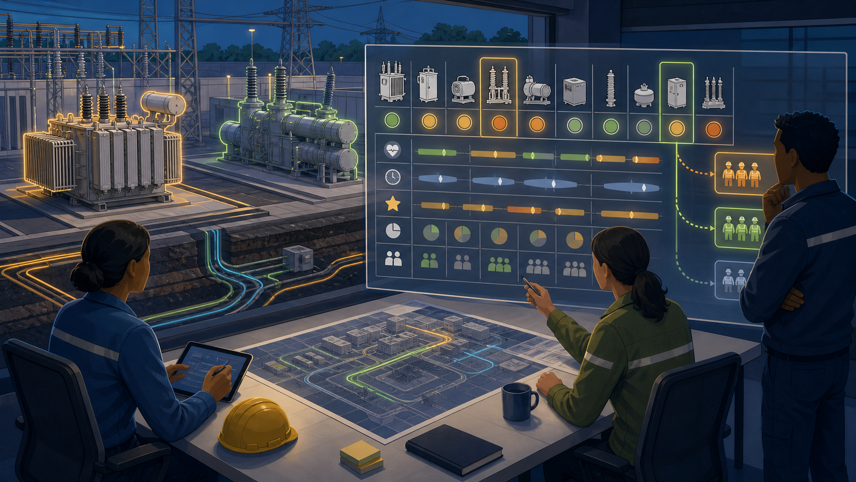
Walk one cycle of the asset management scenario — thermal anomaly detection, Health Index (HI), Weibull-based Remaining Useful Life (RUL), and maintenance schedule optimization for 10 transformers, GIS, and underground cables.
Workshop goal
By the time you finish this Workshop, you will have walked through one full cycle of the following flow inside D.Hub.
- Load a single scenario into portal so that one collection, 11 datasets (7 input + 4 output), 6 code nodes, 5 pipelines, an ontology with 6 entities and 6 relations, a dashboard, and one knowledge are all registered together.
- Inspect 7 inputs across 10 pieces of equipment — 5 transformers (154–765 kV), 3 GIS (170–362 kV), and 2 underground cables (154 kV) — covering master, sensor, inspection, maintenance, DGA, and failure history.
- Execute the 4-algorithm pipeline chain in sequence:
thermal_anomaly_detection— Identify abnormal temperature patterns via Z-score + IQR + CUSUMhealth_index_evaluation— Produce a 0–100 HI score using IEC/IEEE weighted rules and assign A–E gradesreliability_rul_estimation— Estimate Remaining Useful Life (RUL) with confidence intervals via Weibull MLE + operating-condition correctionmaintenance_optimization— Build a priority-ordered maintenance schedule under budget and crew constraints
- Expand a single transformer's subsystem → sensor → inspection → defect → maintenance path in the
HS_Equipmentgraph. - Read the operational view via the
equipment_health_overviewdashboard's 8 widgets.
This is the Predictive Maintenance (PHM) IIoT Workshop. Where the iot Workshop covered anomaly detection → daily rollup, this one extends to lifetime estimation → schedule optimization. Recommended duration: 90 minutes.
Prerequisites
- An engineer account with access to D.Hub portal (Editor or higher)
- ~156 KB of download room for one scenario zip
Finishing the iot Workshop first makes the sensor time series → anomaly detection → daily aggregate basics flow into the 4-algorithm chain naturally.
1. Load the scenario (10 min)
hs_asset_management.zip Download(152 KB)Go to Collections → more (⋯) menu → Import (가져오기) and upload the zip.
Following manifest.json, the import creates the following in order:
- One collection —
hs_asset_management(alias: Power Equipment Asset Management) - 11 datasets — Inputs 7 (
equipment_master,sensor_readings,inspection_records,maintenance_records,dga_analysis,failure_history,operating_conditions), outputs 4 (thermal_anomaly_results,health_index_scores,rul_estimates,maintenance_schedule) - 6 codes (Python) —
thermal_anomaly_detection,health_index_evaluation,reliability_rul_estimation,maintenance_optimization,build_hs_ontology,report_generation - 5 pipelines —
health_assessment,reliability_analysis,maintenance_planning,ontology_materialization,periodic_report - Ontology — 6 entities (
HS_Equipment,HS_Subsystem,HS_Sensor,HS_Inspection,HS_Defect,HS_Maintenance), 6 relations - One knowledge —
equipment_maintenance_manual - One dashboard —
equipment_health_overview(8 widgets)
2. Browse the input data (10 min)
equipment_master (10 rows) — Asset master. Columns: equipment_id (TX-001 ~ TX-005, GIS-001 ~ GIS-003, CBL-001 ~ CBL-002), equipment_type, voltage_kv, commissioned_year, manufacturer, installation_site.
sensor_readings — Sensor time series across 3 measurement types:
- Temperature (
°C, transformer windings/core, GIS compartments) - Partial Discharge PD (
pC, insulation degradation signal) - Gas density (
g/L, SF6 in GIS)
Sampled every 5 minutes. Columns: reading_id, equipment_id, sensor_type, value, recorded_at, quality_flag (OK / WARN / FAULT).
inspection_records — Periodic inspection results. equipment_id, inspection_date, inspector, result_summary, defects_found (array).
maintenance_records — Past maintenance history. equipment_id, maintenance_date, maintenance_type (preventive / corrective / emergency), defect_id, duration_hours, cost.
dga_analysis — Dissolved Gas Analysis (transformers only). Columns: 6 gas concentrations (H2, CH4, C2H6, C2H4, C2H2, CO), sampling_date. Gas ratio patterns are a strong signal of which failure mode is progressing.
failure_history — Training data for Weibull. equipment_id, failure_date, failure_mode, time_to_failure_years. The RUL estimation in §4 fits this distribution.
operating_conditions — Load rate / temperature / humidity. Used for operating-condition correction.
A subtle point — the 7 inputs all have different time resolutions and frequencies: 5 minutes (sensors), daily (DGA), monthly (inspections), ad-hoc (maintenance, failure). The next-step pipelines reconcile these into per equipment / per time window alignment.
3. Thermal anomaly detection + HI evaluation (15 min)
Open the health_assessment pipeline. Two nodes.
thermal_anomaly_detection— Read temperature readings fromsensor_readings, then compute per-equipment per-sensor anomaly scores via Z-score + IQR + CUSUM. Output:thermal_anomaly_resultswith columnsequipment_id,sensor_id,window_start,window_end,zscore,iqr_outlier_flag,cusum_drift,anomaly_score(0–1 composite).health_index_evaluation— Compute HI using IEC 60076 / IEEE C57 weighted rules. Inputs:equipment_master(aging) +thermal_anomaly_results(thermal) +dga_analysis(gas, transformers) +inspection_records(inspection results). Weights are equipment-type specific — transformers weight DGA heavily, GIS weight gas density heavily.
HI score → grade mapping in health_index_evaluation:
| HI score | Grade | Meaning |
|---|---|---|
| 85–100 | A | Normal, new / low-degradation |
| 70–84 | B | Minor degradation |
| 55–69 | C | Mid-stage degradation, monitor closely |
| 40–54 | D | Severe degradation, maintenance priority |
| 0–39 | E | At risk, immediate inspection |
Press Run. When it finishes, open health_index_scores and inspect the 10-equipment HI scores and A–E grade distribution.
4. Weibull-based RUL estimation (15 min)
Open the reliability_analysis pipeline. One node — reliability_rul_estimation reads failure_history + operating_conditions + health_index_scores and produces rul_estimates.
Weibull is the standard reliability model when failure rate changes over time. The script's two stages:
- MLE fitting — Fit Weibull shape parameter β and scale parameter η per equipment type against the
time_to_failure_yearsdistribution infailure_history. - Operating-condition correction — Without correction, all equipment receives the same RUL. The script applies
operating_conditions's load rate / temperature / humidity as correction factors and multiplies in HI as an acceleration factor to estimate RUL given current state.
Output columns of rul_estimates: equipment_id, rul_years (point), rul_lower_5pct, rul_upper_95pct (90% CI), confidence_level, estimation_method.
Press Run. In the preview, confirm both CI columns are populated and that D-grade equipment's rul_years is shorter than the others.
5. Maintenance schedule optimization (15 min)
Open the maintenance_planning pipeline. One node — maintenance_optimization reads rul_estimates + health_index_scores + maintenance_records and produces maintenance_schedule.
Problem statement, in one line: under budget and crew constraints, place the highest-priority equipment into the schedule first. The priority score uses greedy ordering by priority_score = (1 / rul_years_lower_5pct) × HI_weight × cost_factor.
Script parameters:
annual_budget— Annual maintenance budget (seed: 500M KRW)monthly_crew_hours— Available crew hours per month (seed: 320 hours)min_interval_days— Minimum interval between maintenance events on the same equipment (seed: 90 days)
Output columns: equipment_id, scheduled_date, maintenance_type (preventive / corrective), estimated_cost, estimated_hours, priority_score, rationale.
Press Run. Confirm in the preview that D-grade equipment lands in the first month and that the cumulative budget / hours stay within the constraints.
6. Ontology + graph exploration (15 min)
Run ontology_materialization. build_hs_ontology reads 7 inputs + 4 outputs in batch mode and lands the 6 entities + 6 relations in upsert mode.
| Entity | Key | Key attributes |
|---|---|---|
HS_Equipment | equipment_id | equipment_type, voltage_kv, latest_hi_score, latest_grade, rul_years, scheduled_maintenance_count |
HS_Subsystem | subsystem_id | parent_equipment_id, subsystem_type |
HS_Sensor | sensor_id | parent_equipment_id, sensor_type, reading_count, latest_recorded_at |
HS_Inspection | inspection_id | equipment_id, inspection_date, result_summary |
HS_Defect | defect_id | equipment_id, severity, detected_at |
HS_Maintenance | maintenance_id | equipment_id, maintenance_date, cost, defect_id |
Relations × 6: HAS_SUBSYSTEM, MONITORED_BY (equipment → sensor), INSPECTED_ON, HAS_DEFECT, DETECTED_BY (inspection → defect), REPAIRED_BY (defect → maintenance).
In the Graph explorer, surface one equipment's vertical decomposition and horizontal history in one view.
MATCH (e:HS_Equipment {equipment_id: 'TX-003'})
OPTIONAL MATCH (e)-[:HAS_SUBSYSTEM]->(s:HS_Subsystem)
OPTIONAL MATCH (e)-[:MONITORED_BY]->(sn:HS_Sensor)
OPTIONAL MATCH (e)-[:HAS_DEFECT]->(d:HS_Defect)-[:REPAIRED_BY]->(m:HS_Maintenance)
RETURN e, s, sn, d, m
One transformer's subsystems + sensors + defects + maintenance fan out on one screen. A single-asset lifecycle compressed into a graph view.
7. Dashboard + next steps (10 min)
The equipment_health_overview (alias: Equipment Health Overview) dashboard's 8 widgets summarize the operational view, spreading evenly across the 4 output datasets.
- Managed equipment count (statistic) —
COUNT(DISTINCT equipment_id)onequipment_master - Average Health Index (statistic) —
AVG(overall_hi)onhealth_index_scores - Equipment with anomaly detected (statistic) —
anomaly_flag = truecount onthermal_anomaly_results - Equipment with RUL < 2 years (statistic) —
rul_estimate_years < 2.0count onrul_estimates - HI by equipment (bar) —
equipment_id×overall_hionhealth_index_scores, ascending - RUL years by equipment (bar) —
equipment_id×rul_estimate_yearsonrul_estimates, ascending - Equipment by health grade (data table) — Counts per
gradeonhealth_index_scores(A–E distribution) - Maintenance schedule (data table, Top 20) —
equipment_id·scheduled_day·maintenance_type·estimated_cost·priority_score, by priority descending
The 4-stat headline drives the operational view. If average HI is falling, anomaly count is growing, and RUL < 2yr count is rising together, that becomes the immediate budget / crew reallocation signal. The two bars show which equipment sits at either extreme; the two tables drive next actions (grade-based inspection intensification, maintenance order generation).
Each widget reads from one of the 4 output datasets directly, so a single pipeline re-run propagates across the whole dashboard immediately.
Next directions:
- The Engineer Path Pipeline scheduling lesson — register the 4 pipelines on the operational cadence (
health_assessmentdaily 02:00,reliability_analysisMonday 03:00,maintenance_planningMonday 04:00,ontology_materializationMonday 05:00). - Compare with the
iotWorkshop — feel the difference between the short-cycle (anomaly detection) and the long-cycle (lifetime estimation) within the same IIoT domain.
Verification checklist
- The
hs_asset_managementcollection holds 7 inputs + 4 outputs. - After
health_assessment, the 10 pieces of equipment inhealth_index_scoresdistribute across A–E grades, and the DGA-troubled transformer (seedTX-003) drops to grade D. - After
reliability_analysis, every row ofrul_estimateshas populated CI columns (rul_lower_5pct,rul_upper_95pct). - After
maintenance_planning, the cumulative first-month cost onmaintenance_schedulestays withinannual_budget / 12(constraint satisfaction). - In the Graph explorer, starting from one
HS_Equipmentyou can expand 4 neighbor types (Subsystem/Sensor/Defect/Maintenance) on one screen.